In the United States, Medicare is a single-payer, national social insurance program administered by the U.S. federal government since 1966. Healthcare is an increasingly important issue for many Americans; the Centers for Medicare and Medicaid Services estimate over 41 million Americans were enrolled in Medicare prescription drug coverage programs as of October 2016. It provides health insurance for Americans aged 65 and older who have worked and paid into the system through the payroll tax. Unfortunately, with modern US Healthcare programs’ complexity and sophistication, fraud losses in healthcare cost US taxpayers a staggering amount, to quote from the Justice Department,

“Health care fraud costs the United States tens of billions of dollars each year.
Some estimates put the figure close to $100 billion a year. It is a rising threat,
with national health care expenditures estimated to exceed $3 trillion in 2014.”
- U.S. Department of Justice

This project aims to tackle this data using a data-driven approach, particularly we hope to:

●     Detect patterns of fraud Medicare providers.

●     Build classification models to detect these providers.

Solutions to all problems start with gathering data and seeing the big picture through big data analytics lens, here I employed a combination of data including CMS Medicare 2014 Part D data from Google BigQuery, Medicare Exclusion list from the Office of Inspector General, and a geographical dataset.

Topics that will be covered using these datasets include

1. Exploration of Medicare drug prescription and cost across states
2. Exploration of excluded drug providers
3. Feature selection and engineering
4. Selection and optimization of classifications models

Data source:   1. https://cloud.google.com/bigquery/public-data/medicare

                        2. https://oig.hhs.gov/exclusions/exclusions_list.asp#instruct

                        3. https://simplemaps.com/data/us-cities

Medicare Part D plans are offered by insurance companies and other private companies approved by Medicare. The analyses and conclusion from the current study are expected to be helpful for just these organizations, but also those that oversee Medicare program including federal centers such as Department of Justice and Department of Health and Human Services.

2.   Dataset Description and Cleaning

The Medicare part D data set contains over 23 million observations of each provider with each drug (~3GB). The features included in the dataset are npi (national provider identifier), provider city, provider state, specialty description, description flag, drug name, generic name, beneficiary (bene) count, total claim count, total day supply, and total drug cost for all Medicare beneficiaries and beneficiaries whose ages are greater than 65. As shown in Table 1, we can see that the statistics of just 1/10^th of the dataset (~2.3 million observations) is similar to the whole dataset and therefore sufficient for data exploration and developing classification model. For the exclusion dataset from the Department of Justice, it contains the npi, names, and location of the excluded provider. From which we will only use the npi to label the provider in the medicare dataset whether the observation is from a fraud provider or from typical provider.

Table 1. The basic statistics of the whole dataset and the sample (1/10^th) we used.

For data wrangling steps, several data cleaning were applied including

·         Checking for NaN (no NaN were found in the interested columns of the original dataset).

·         Managing address location text data.

·         Combining data from different datasets.

·         Grouping data by States, drug providers, costs, etc.

·         Data preprocessing: creating features that weren’t readily available in the data (ratios).

The raw data does not contain missing values. However, by grouping data by drug sale. Certain providers do not have any sale, which makes a feature drug sale per provider become infinity (NaN). These providers were removed as they do not sell any drug anyway. There were some outliers, but we do not delete them as we are trying to detect anomalies in sales, and these outliers maybe the anomaly we are looking for.

3.   Initial findings from exploratory analysis

3.1        Data Story

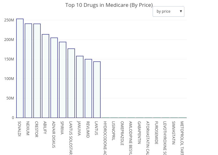
Fig. 1. The top 10 drugs prescribed in Medicare by total cost.  

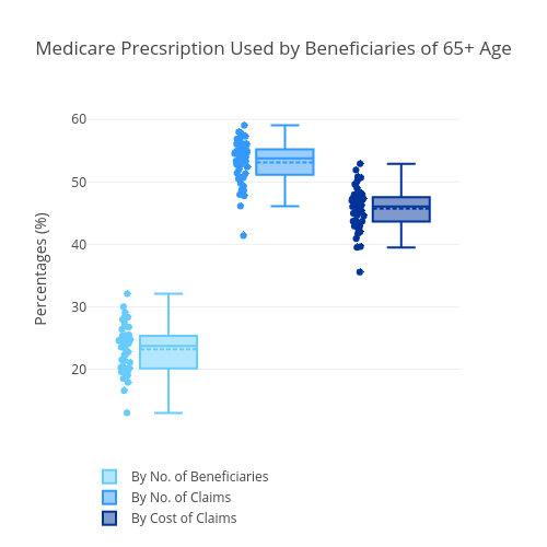
Fig. 2. The portion of Medicare used by 65+ beneficiaries.

Medicare is the federal health insurance program for: People who are 65 or older. Certain younger people with disabilities. People with End-Stage Renal Disease (permanent kidney failure requiring dialysis or a transplant, sometimes called ESRD). Medicare Part D includes prescription drug coverage to original Medicare some Medicare Cost Plans, some Medicare Private-Fee-for-Service Plans, Medicare Medical Savings Account Plans, available for.

By looking just at the Medicare dataset itself, we can draw some interesting facts out of the data. In 2014, a total of $ 90 billion from 83,000 providers with 2695 unique drugs were prescribed using Medicare. By the cost of total prescriptions, the drug with the highest total cost is Sovaldi, a medication for Hepatitis C (Fig. 1). However, by amount of prescriptions, Hydrocodone - a narcotic pain relieving drug - is the most prescribed drug (figure not shown). Across the States, only 24% of the beneficiaries are of 65+ ages (the rest are disabled beneficiaries). However, beneficiaries with 65+ age contributed to more than 45% of the cost in Medicare prescription Fig.2.

Interestingly, there is a huge disparity in the Medicare prescription cost across the states, with States near the West Coast tend to be significantly cheaper Fig. 3. Although this will not be the focus of the current study, it is an excellent starting point to understand and investigate geographic and racial and ethnic differences in health outcomes. This information may be used to inform policy decisions and to target populations and geographies for potential interventions.

Fig. 3. The average cost of drug prescription in different cities showing disparities across United States.

Fraud Medicare provider is listed in an exclusion list by the Department of Justice due to several reasons including:

1. Fraud by claiming of Medicare reimbursement to which the claimant is not entitled.

2. Offenses related to the delivery of items or services under Medicare.

3. Patient abuse or neglect

4. Unlawful manufacture, distribution, prescription, or dispensing of controlled substances.

From the combination of the datasets, fraud provider associated with the Part D Medicare accounts to approximately 0.2%, of all providers and prescribed at least $200 million worth of drugs in the year 2014 alone. From exploratory data analyses, we found that there is no correlation in the provider’s specialty between typical and fraud providers. This feature of the provider is therefore not worth it for identification of fraud providers.

Interestingly, by ranking the top 10 most prescribed drugs again, but from only the fraud providers (Fig. 4), a very unique set of drug trends are revealed. More than 5 narcotics, including OxyContin (Fig. 5), Oxymorphone, Morphine, Oxycodone HCL, and Oxycodone-acetaminophen are on the list compared to just 1 from all providers shown in Fig. 1 (Hydrocodone). Suggesting that fraud providers tend to sell significantly more narcotics and could be useful as a feature for classification purposes. However, feature engineering needs to be applied.

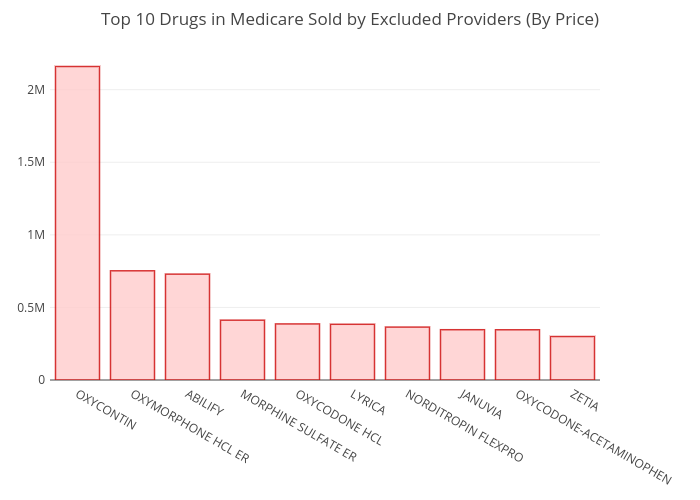
Fig. 4. The top 10 drugs prescribed by fraud providers. .

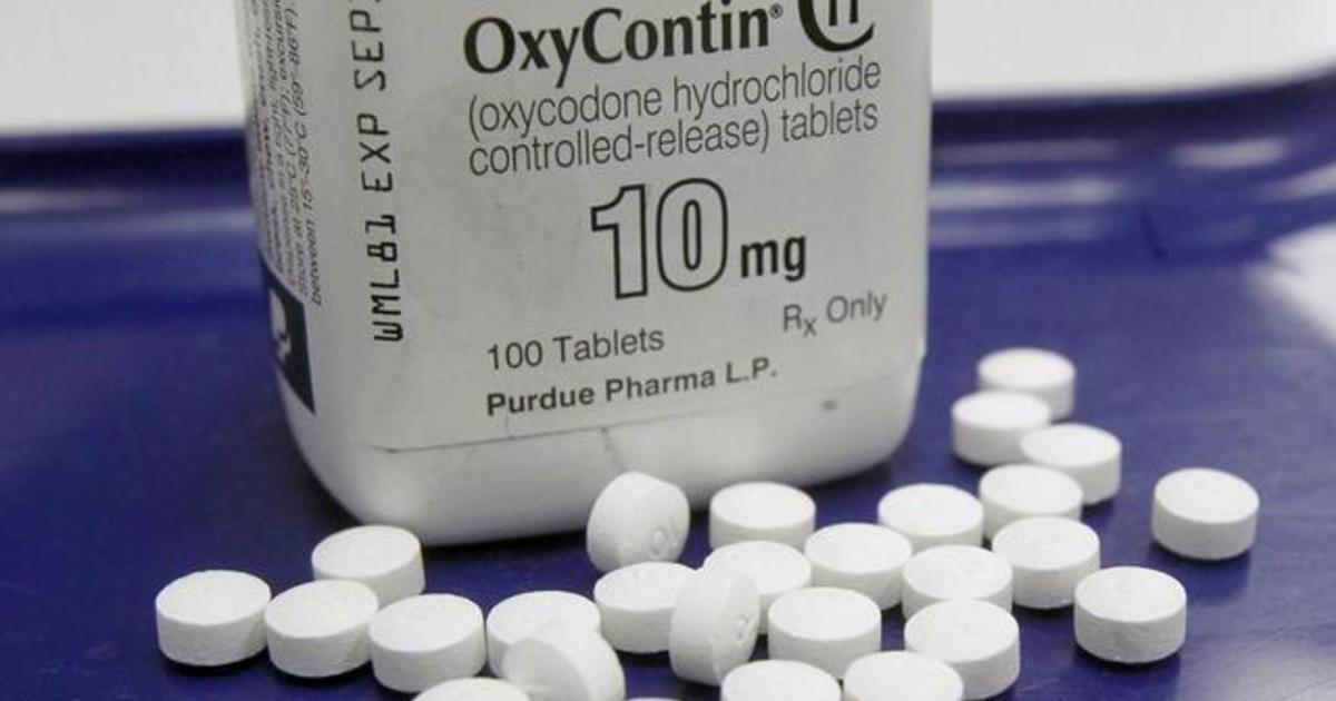
Fig. 5. The top selling narcotics drug (OxyContin).¹

Furthermore, by looking into a statistic overview of the sale of narcotics between typical and fraud drug providers, we found a more convincing evidence. In Fig. 6, an average total sale of generic (in blue) and narcotic (in red) drugs are shown for typical and fraud providers. Although both typical and fraud providers sell generic drugs at about the same cost ($3900), fraud providers’ sales of narcotics skyrocketed to over $41,000 on average, while typical providers have narcotic sale similar to other drugs. The total cost of narcotics by fraud providers are high primarily due to the sale amount. The amount is depicted as a size of the bubble in Fig. 6. This difference in sale behavior between typical and fraud provider will be further investigated in the next section; however, this shows that it is an interesting feature that can be leveraged for machine learning models. As drug cost is currently just one feature in the dataset, how we expand this feature into more independent variables will be discussed in Section 4.

Fig. 6. Average total Medicare cost per beneficiary by excluded (fraud) and non-excluded (typical) providers.

          3.2 Inferential Statistics

In this section, we provide more statistical supports to the conclusion drawn from data analysis in the previous section.

Fig. 7. Average amount of generic drugs (left) and narcotics (right) plotted against the average total sale (in $) of typical (light blue) and fraud providers (red).

1. Sale Behaviors

Here, we will look more into the statistics of this anomalies. The scatter plot of the drug/narcotics amount and cost sale from typical and fraud providers in Fig. 7 showed that there is a huge overlaps and definitely inseparable. However, we can observe that in narcotics only plot (Fig. 7 right), the trend is more slightly more scattered. To determine that population’s mean of the cost from fraud and typical providers are in fact significantly different, we applied one-way ANOVA test.

The results showed that the null hypothesis that fraud providers sell all drugs with the similar total cost as typical provider has a p-value of 0.6987, therefore, we do NOT reject the hypothesis. On the other hand, the null hypothesis that fraud providers sell narcotics with the same total cost as typical provider has a p-value of 0.0000, therefore, we REJECT the hypothesis. This supports that there is a difference on average; however, as can be seen in Fig. 7 that using this feature (total sale) directly does not suffice for any model to separate it. Therefore, we need increase the dimension of the data by constructing more independent variables out of the existing information, which will be discussed in the Section 4.

*narcotics includes ['OXYCONTIN', 'OXYMORPHONE HCL ER', 'MORPHINE SULFATE ER', 'OXYCODONE HCL', 'OXYCODONE-ACETAMINOPHEN', 'FENTORA', 'SUBSYS', 'HYDROCODONE-ACETAMINOPHEN', 'SUBOXONE', 'OPANA ER', 'HYDROCODONE-ACETAMINOPHEN'], which are among the top 25 of the most sold drugs by fraud providers

2. Specialty of Fraud Providers

Fig. 8. The percentages of excluded (fraud) and non-excluded (typical) Medicare providers’ specialties.

The second objective is to determine if there is any correlation between the specialty of providers and whether that provider is a fraud one. For this objective, we employed Spearman’s correlation because it is suitable for comparison between two categorical classes and it does not assume the datasets are normally distributed. The correlation between providers' specialty and whether the provider is fraud is 0.0023 with a p-value of 0.0003. The low p-value indicates that the null hypothesis that specialty and whether the providers are fraud are uncorrelated, is rejected. However, the correlation value was virtually 0, which means that the correlation would not be necessarily useful, and hence we would not leverage this feature for the classification model.

4. Results and In-depth analysis using machine learning

            Prior to employing machine learning models. We performed several feature engineering to the original data. First, we need to create more independent variables out of the current useful features, drug name and total sale. We expanded these two features by creating a matrix with providers as indices and each column of the row is a drug name with a value of sale portion of that drug. In this way, we construct independent features that reflect sale behavior of each provider. In should be noted that since there are more than 2 million providers. It does not make sense to use all drugs as a part of feature construction. Herein, we only used drugs that were sold (at least once) by fraud providers. This reduces the number of unique drugs from 2191 to 553 types. The example of the resulting table is shown in Table 2.

Table 2. Example of the features generated from drug names and its sale portion for different providers.

                As one might have expected, the generated features that consist of 553 columns are low-rank matrix and is filled mostly with zeros. To get rid of unnecessary features as well as avoiding the curse of dimensionalities, we applied principal component analysis (PCA) to the data. In Fig. 9, it is shown that by using 2 and 3 components, the variances explained are 8% and 10% respectively. This may sound like a small number, but consider there are more than 553 features, this means that the rest of the 550 features would contribute to less than 0.17% each. This implies that the rest of the components may be negligible.

Fig. 9. Explained variance using 2 and 3 principal components.

            To test if the engineered data could be better separated than the original ones as shown in Fig. 7 (right), scatter plots of the data with 2 and 3 components with label are shown in Fig. 10. In both of these figures, we can observe the agglomeration of the fraud providers, although not totally separated from typical providers. In the case where only 2 principal components were used, majority of the fraud providers exhibited PC2 lower than 0.1, with significant amount of those data points lying in a negative PC1 and negative PC2 region. Similarly, in the case of 3 components we can see that most fraud providers exhibited PC2 of lower than 0.2 and significant amount of those data points lying in a negative PC1 and negative PC3 region. This shows a promising result that machine learning models may be able to classify these points. However, judging from the shape and degree of overlaps of the data, it is expected that decision tree-based algorithms would do well in this situation. Not only because the data is highly non-linear, non-Gaussian, but the amount of red data point (fraud providers) is significantly less than the light blue ones (typical providers).

Fig. 10. Labelled scatter plot of typical (light blue) and fraud (red) providers plotted in its corresponding 2 principal components (left) or 3 principal components (right).

In summary, the number of typical providers is 486675 providers, as opposed to just 566 fraud providers. This would a heavy class imbalance for our classification model that even a tree-based algorithm may not be able to identify. To address this problem, we investigated several bootstrapping technique including up-sampling, down-sampling, and combination of both using an ensemble method, random forest with 50 trees, as a benchmarking algorithm. The bootstrapped samples will be separated 66/33 for training and test set. The results are then judged based on confusion matrices. It should be noted here that simple accuracy is not used as a scoring metric because even if the classification model predict that all providers are typical, the accuracy will still be above 98%. Using confusion matrix, which encompass both true/false positive and negative, enable us to clearly see where the model performs best and which needs to be improved.

Table 3. The confusion matrix results with precision and recall score for no and different types of bootstrapping methods. The results are obtained using random forest algorithm with 50 trees.

            From Table 2, we can see that bootstrapping to increase the number of fraud providers is an important step. On the major column, we can see that with no resampling at all, the random forest algorithm can only capture the fraud provider in the training set, while it utterly failed to detect a single fraud provider in the test set. By up-sampling the fraud providers by about 10 folds, the algorithm performed significantly better, with a very precision of 98% and satisfactory recall of 77% in the test set, which is also very close to the training set results. However, down sampling data by ten times (down-sampling the number of typical providers) did not yield improved results. On the contrary, the outcomes are slightly below no sampling results. It should be noted here that down-sampling further to 100 folds were investigated and the results exacerbate. Lastly, the results from combination of these two techniques showed an improved in recall, but lower precision compared to up-sampling only method.

For the present study, we favor a conservative approach and choose to perform only up-sampling. We chose to maintain high-precision over improved recall because we want to be able to identify with high precision which providers are fraud. Moreover, lower precision means

significant more numbers of typical providers will be classified as fraud providers since there are way more of them than fraud providers. This would make verification process troublesome.

Fig. 11.  F1 score from different classification models.    

Fig. 12. Receiver operating characteristics (ROC) and area under curve (AUC) of each classification model.

            We first use data with 2 principal components and 5 fold cross validations to screen for the potential classifiers. In this step we used two criteria to judge the performance of classification models. These include F1 score and area under curve (AUC) of the receiver operating characteristics (ROC). Both of which, unlike accuracy, are metrics that take into account the effect of true/false positive and negative results. F1 score is defined as 2*(precision * recall) / (precision + recall), whereas ROC is the curve between false positive rate and true positive rate. Therefore, AUC is equal to the probability that a classifier will rank a randomly chosen positive instance higher than a randomly chosen negative one ‒ the higher the better.

The results in Fig. 11 and Fig. 12 showed that random forest and extra trees algorithm performed the best among all studied models including naïve Bayes, K nearest neighbors, Gaussian SVC, Adaboost (decision tree base classifier), gradient boosting. Naïve Bayes, SVC, and Adaboost were not able to capture recall and hence the F1 score becomes zero (Fig. 11). Note that most models that yielded descent scores are based on "decision tree algorithms". This is because these trees are able to cope with class imbalance better by their hierarchical structure that allows them to learn signals from both classes given sufficient branches.² The results showed that extra trees method is slightly better than random forest with F1 and AUC of 0.873 and 0.98 versus 0.869 and 0.98 from random forest. Here, it is worth mentioning the difference between these two methods. Random forest is a commonly used ensemble method for many applications and it functions by, as the name suggest, having numbers of trees each takes in a different number of features and vote. The process is repeated with bootstrap sampling so that each tree is exposed to more data. Extra trees, short from extremely randomized tree, drops the idea of using bootstrapping copies, and with the split chosen at random from the range of values in the sample at each split, resulting in higher number of leaves. It is expected that extra trees tend to perform worse when there is a high number of noisy features (in high dimensional data-sets).³

Fig. 13.  F1 score of optimized extra tree model with increased number of principal components.

To further increase the performance, we optimized the extra trees method using grid search over different parameters including number of trees, number of features in each tree, number of samples required to split nodes. The optimized model required up to 200 trees instead of just 50 trees in the original extra tree model. Lastly, the results were optimized by increasing the number of principal components. We can see that just 3 components are sufficient to obtain an F1 score of 0.874 (with 0.986 precision and 0.784 recall), which is considerably high.

            For future studies, there are several ways that could be used to improve the performance of the model. For example, by incorporating Medicare Provider Utilization and Payment Data (https://www.cms.gov/Research-Statistics-Data-and-Systems/Statistics-Trends-and-Reports /Medicare-Provider-Charge-Data/Part-D-Prescriber.html), which contains information about which providers were paid by which drug companies and by how much in order to promote their drug sales. This is required by law. Unfortunately, the identifier provided in the payment dataset is purposefully altered so that one could not match with the identifier in the Medicare and exclusion dataset (npi). Although there are venues that one could back track these numbers, the process is heavily time consuming and potentially illegal. Therefore, this study did not pursue the use of payment dataset to add more features to it. Applying graph theory to these would likely yield very interesting insight as well.

5. Conclusion

            In conclusion, the present studies employ multiple big dataset in Medicare prescription to explore the Medicare drug prescription in the U.S. More importantly, we highlighted the difference in sale behaviors between typical providers and fraud providers. Fraud providers sells drugs in different ratios and total cost from typical providers. They tend to sell more narcotics at higher cost. In total, health care fraud costs the United States tens of billions of dollars each year. To detect these fraud drug providers, we performed feature engineering and screened different classification models. The random forest and extra trees results were found to be successful due to their bootstrapping and hierarchical structure that enable them to capture class imbalance better. The optimized extra trees model yielded F1 score of over 0.874 (with 0.986 precision and 0.784 recall). Further improvement in the future could be obtained by incorporating currently prohibited payment data.

6. References

1. https://www.cbsnews.com/news/purdue-oxycontin-maker-to-stop-promoting-drug-to-doctors-amid-opioid-epidemic/  Access: Jun 2018

2. Liaw, A., & Wiener, M. (2002). Classification and regression by random forest. R news, 2(3), 18-22.

3. Geurts, P., Ernst, D., & Wehenkel, L. (2006). Extremely randomized trees. Machine learning, 63(1), 3-42.